Inquire: Call 0086-755-23203480, or reach out via the form below/your sales contact to discuss our design, manufacturing, and assembly capabilities.
Quote: Email your PCB files to Sales@pcbsync.com (Preferred for large files) or submit online. We will contact you promptly. Please ensure your email is correct.
Notes: For PCB fabrication, we require PCB design file in Gerber RS-274X format (most preferred), *.PCB/DDB (Protel, inform your program version) format or *.BRD (Eagle) format. For PCB assembly, we require PCB design file in above mentioned format, drilling file and BOM. Click to download BOM template To avoid file missing, please include all files into one folder and compress it into .zip or .rar format.
After two decades of working with circuit boards—from simple sensor interfaces to complex multi-layer telecommunications equipment—I’ve learned that understanding digital integrated circuits is fundamental to every electronics project. Whether you’re selecting a simple logic gate for signal conditioning or specifying a microcontroller for an embedded system, knowing the types of digital IC available shapes every design decision you make.
This digital IC guide walks through the complete landscape of digital integrated circuits, from basic logic families to advanced programmable devices. I’ll cover what matters for practical PCB design: selection criteria, interface considerations, and the tradeoffs you’ll encounter in real projects.
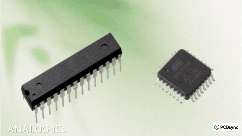
Digital integrated circuits are semiconductor devices that process discrete binary signals—logical ones and zeros represented by voltage levels. Unlike analog ICs that handle continuous signals, digital integrated circuits operate with just two defined states: HIGH (typically 3.3V or 5V) and LOW (typically 0V or ground).
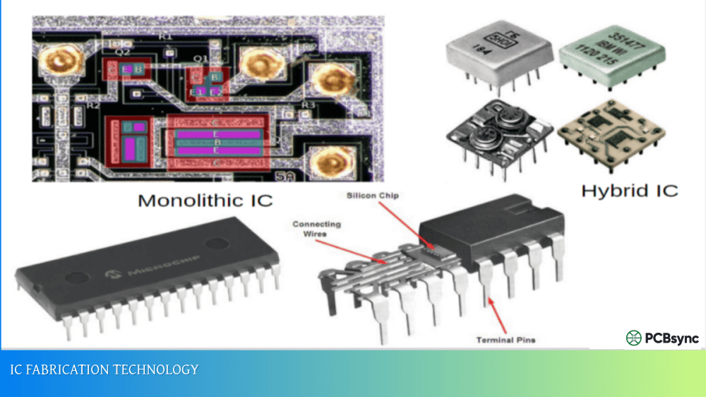
Every digital IC you’ll encounter contains some combination of transistors, resistors, and capacitors fabricated on a silicon substrate. These components are interconnected within the chip to perform specific logical operations—from simple AND/OR gates to complex microprocessors containing billions of transistors.
The semiconductor material forms the foundation of all digital integrated circuits. Silicon remains dominant due to its excellent semiconductor properties and mature manufacturing processes. The fabrication process uses photolithography to create microscopic transistor structures, with modern processes achieving feature sizes below 5 nanometers.
The key characteristics that define any digital integrated circuit include propagation delay (how fast signals move through the device), power consumption (static and dynamic), noise margin (how much interference the device tolerates), and fan-out (how many inputs a single output can drive). These parameters directly influence your PCB layout, power supply design, and signal integrity strategy.
How Digital ICs Process Information
Digital circuits represent information using binary numbers. Each bit corresponds to a voltage level—typically above a threshold for logic “1” and below a threshold for logic “0”. The gap between these thresholds provides noise immunity, allowing digital circuits to operate reliably in electrically noisy environments.
When a digital input transitions between states, the output responds after a characteristic propagation delay. This delay accumulates through chains of logic gates, ultimately limiting system operating frequency. Understanding propagation delay is essential when designing timing-critical circuits like clock distribution networks or high-speed data interfaces.
Classification of Digital Integrated Circuits
Types of digital IC can be organized several ways: by function, by fabrication technology, by logic family, or by integration level. Each classification system serves different purposes when you’re selecting components for a design.
Classification by Function
Functionally, digital ICs fall into these major categories:
Logic ICs: Perform basic Boolean operations (AND, OR, NOT, NAND, NOR, XOR). These are the fundamental building blocks of all digital systems. Every complex digital function ultimately reduces to combinations of these primitive operations.
Memory ICs: Store digital data either temporarily (RAM) or permanently (ROM, Flash). Includes SRAM, DRAM, EEPROM, and various flash memory types. Memory capacity has grown exponentially, with modern chips storing terabits of data.
Processor ICs: Execute programmed instructions, including microprocessors (CPUs), microcontrollers (MCUs), and digital signal processors (DSPs). These devices transformed electronics by enabling software-defined functionality.
Programmable Logic ICs: User-configurable devices including PLDs, CPLDs, and FPGAs. These chips blur the line between hardware and software, allowing designers to implement custom digital functions without manufacturing custom silicon.
Interface ICs: Handle communication between different digital systems or between digital and analog domains—includes bus transceivers, level shifters, and protocol controllers. These devices manage the electrical and protocol translation that allows diverse components to communicate.
Classification by Integration Level
The number of transistors packed onto a single chip defines the integration level. This classification reflects the historical progression of semiconductor manufacturing capability:
Integration Level
Abbreviation
Transistor Count
Gate Equivalent
Typical Examples
Small Scale
SSI
1-100
1-10 gates
Basic logic gates (7400 series NAND, NOR)
Medium Scale
MSI
100-1,000
10-100 gates
Multiplexers, decoders, counters, adders
Large Scale
LSI
1,000-10,000
100-1,000 gates
Simple microprocessors, small memories
Very Large Scale
VLSI
10,000-1,000,000
1,000-100,000 gates
Advanced microprocessors, large memories
Ultra Large Scale
ULSI
1,000,000+
100,000+ gates
Modern CPUs, GPUs, SoCs, FPGAs
When I started in this industry, a “complex” design might use a handful of LSI chips. Today, a single smartphone SoC contains more transistors than all the computers that existed in 1970 combined. Modern processor chips exceed 50 billion transistors—a scale that would have seemed impossible just two decades ago.
The progression from SSI to ULSI follows Moore’s Law—the observation that transistor density doubles approximately every two years. While physical limits are approaching, innovations in 3D stacking and advanced packaging continue extending this trend.
Classification by Manufacturing Technology
The fabrication process significantly impacts device characteristics:
Bipolar Technology: Uses bipolar junction transistors (BJTs). Offers high speed and strong output drive but consumes more power. TTL and ECL logic families use bipolar technology.
MOS Technology: Uses metal-oxide-semiconductor field-effect transistors (MOSFETs). Lower power consumption than bipolar, enabling higher integration densities. NMOS uses only n-channel devices; PMOS uses only p-channel devices.
CMOS Technology: Uses complementary pairs of NMOS and PMOS transistors. Achieves extremely low static power consumption because current flows only during switching transitions. Dominates modern digital IC manufacturing.
BiCMOS Technology: Combines bipolar and CMOS on the same substrate. Leverages bipolar’s drive strength with CMOS’s low power consumption. Used in high-performance interface circuits.
Digital Logic Families: The Technology Foundation
The logic family determines how a digital IC is fabricated and, consequently, its electrical characteristics. Selecting the appropriate logic family affects power consumption, speed, noise immunity, and interface compatibility throughout your design.
TTL: Transistor-Transistor Logic
TTL was the workhorse of digital design from the late 1960s through the 1980s. Using bipolar junction transistors (BJTs), TTL devices operate from a 5V supply with well-defined voltage thresholds.
The 7400 series remains the most recognized TTL family. Introduced by Texas Instruments in 1966, this family established pinout standards still used today. Within this series, you’ll encounter several sub-families optimized for different applications:
Sub-Family
Prefix
Speed
Power
Primary Use Case
Standard
74xx
Moderate
High
Original TTL, legacy systems
Low Power
74Lxx
Slow
Low
Battery applications (obsolete)
Schottky
74Sxx
Fast
Higher
High-speed computing
Low Power Schottky
74LSxx
Moderate
Moderate
General purpose, widely used
Advanced Low Power Schottky
74ALSxx
Fast
Low
Improved 74LS replacement
Fast
74Fxx
Very Fast
Moderate
High-speed bus interfaces
Advanced Schottky
74ASxx
Very Fast
High
Maximum bipolar performance
From a PCB design perspective, TTL’s relatively high current requirements (compared to CMOS) demand attention to power distribution. Each gate draws milliamps even when not switching, so designs with hundreds of TTL gates need robust power planes and adequate decoupling. I’ve debugged countless boards where insufficient decoupling caused mysterious logic glitches—always use at least 0.1µF per device, placed as close to the VCC pin as physically possible.
TTL outputs use a “totem-pole” configuration with two transistors stacked between VCC and ground. This structure provides strong drive in both HIGH and LOW states but cannot be directly connected to other outputs (wire-OR configurations require open-collector variants like the 7401).
CMOS: Complementary Metal-Oxide Semiconductor
CMOS technology uses complementary pairs of n-channel and p-channel MOSFETs. This architecture draws significant current only during switching transitions, making CMOS dramatically more power-efficient than TTL for most applications.
Key CMOS Characteristics:
Supply voltage: 3V to 15V (traditional), 1.8V to 5V (modern)
Logic thresholds: Proportional to supply voltage (typically 30% and 70% of VDD)
Static power consumption: Nanowatts per gate
Dynamic power consumption: Proportional to frequency and capacitance
Excellent noise immunity (nearly half of supply voltage)
High input impedance (essentially zero DC input current)
The 4000 series was the original CMOS family, operating from 3V to 15V supplies. Developed by RCA in the late 1960s, these devices offered unprecedented flexibility in supply voltage at the cost of slower operation. While still available, the 4000 series has largely been superseded by faster families:
Sub-Family
Prefix
Supply Range
Speed
TTL Compatible
Best Application
Original CMOS
4xxx
3-15V
Slow
No
Wide voltage range needs
High-Speed CMOS
74HCxx
2-6V
Fast
No
General CMOS logic
High-Speed CMOS (TTL input)
74HCTxx
5V
Fast
Yes
Mixed TTL/CMOS systems
Advanced CMOS
74ACxx
2-6V
Very Fast
No
High-speed CMOS
Advanced CMOS (TTL input)
74ACTxx
5V
Very Fast
Yes
High-speed mixed systems
Low Voltage CMOS
74LVCxx
1.65-3.6V
Very Fast
Partial
3.3V and lower systems
Low Voltage (TTL)
74LVTxx
3.3V
Very Fast
Yes
3.3V with 5V tolerance
For modern designs, I almost always default to 74HC or 74LVC series devices. The power savings are substantial—a board that might draw 500mA with TTL logic could drop to under 50mA with equivalent CMOS devices, not counting static current which becomes negligible.
CMOS technology has one significant vulnerability: electrostatic discharge (ESD). The thin gate oxide that enables CMOS’s excellent characteristics can be destroyed by static electricity. Modern devices include protection diodes, but handling precautions remain important during assembly.
ECL: Emitter-Coupled Logic
ECL represents the high-performance extreme of bipolar logic. By operating transistors in their linear (non-saturated) region, ECL achieves switching speeds impossible with saturated logic.
Constant current consumption (no supply current spikes)
ECL finds application in high-frequency communications, test equipment, and anywhere nanosecond timing matters. The tradeoff is significant: ECL devices consume substantial power and require careful PCB layout practices to manage the small voltage swings and high-speed edges.
The constant current draw of ECL provides one unexpected benefit: minimal power supply noise. Unlike CMOS where current spikes occur at each transition, ECL current remains steady regardless of switching activity. This characteristic makes ECL attractive for mixed-signal systems where digital noise might corrupt sensitive analog circuits.
For most commercial and industrial applications, CMOS has effectively replaced ECL. However, ECL derivatives like PECL (Positive ECL) and LVPECL (Low Voltage PECL) remain essential for multi-gigabit serial interfaces and precision timing circuits. Modern high-speed serial standards like LVDS evolved from ECL concepts.
BiCMOS: Combining the Best of Both Technologies
BiCMOS technology combines bipolar and CMOS transistors on the same substrate, leveraging the drive strength of bipolar devices with the low power consumption of CMOS. This hybrid approach appears in high-performance logic families like 74ABT and 74LVT.
BiCMOS offers excellent output drive capability while maintaining reasonable power consumption—useful when you need to drive long traces, terminated transmission lines, or multiple loads without external buffering.
The 74ABT family delivers 24mA output drive with CMOS-level power consumption—a combination impossible with either technology alone. For bus interfaces and clock distribution, BiCMOS often provides the optimal solution.
Digital Logic Family Comparison Table
This comprehensive table summarizes the practical characteristics you’ll consider when selecting a logic family for your design:
Parameter
TTL (74LS)
CMOS (74HC)
CMOS (74LVC)
ECL
BiCMOS (74ABT)
Supply Voltage
5V
2-6V
1.65-3.6V
-5.2V
5V
Propagation Delay
10ns
8ns
4ns
1ns
3ns
Static Power (per gate)
2mW
~10nW
~10nW
25mW
0.5mW
Dynamic Power
Moderate
Low
Low
High
Moderate
Fan-out
10
50
50
10
25
Noise Margin
0.4V
~1.5V
~0.7V
0.15V
0.7V
Output Drive (IOH/IOL)
0.4/8mA
4/4mA
24/24mA
50mA
24/24mA
Input Current
0.4mA
~1µA
~1µA
265µA
~1µA
ESD Sensitivity
Low
High
Moderate
Low
Moderate
Types of Digital ICs by Function
Let me walk through the major functional categories of digital integrated circuits you’ll encounter in practical designs.
Standard Logic ICs
Standard logic ICs implement basic Boolean functions. These remain essential building blocks even in an era of programmable logic, particularly for glue logic, signal conditioning, and simple control functions where a dedicated IC costs less and consumes less power than configuring an FPGA.
Common Standard Logic Functions:
Function
Example Part
Gates/Package
Description
Inverter (NOT)
74HC04
6
Hex inverter
Buffer
74HC34
6
Hex non-inverting buffer
AND Gate
74HC08
4
Quad 2-input AND
OR Gate
74HC32
4
Quad 2-input OR
NAND Gate
74HC00
4
Quad 2-input NAND
NOR Gate
74HC02
4
Quad 2-input NOR
XOR Gate
74HC86
4
Quad 2-input XOR
Tri-State Buffer
74HC244
8
Octal buffer with enable
Schmitt Trigger
74HC14
6
Hex inverter with hysteresis
AND-OR-Invert
74HC51
2
Dual 2-wide 2-input AOI
In my experience, Schmitt trigger inputs (like the 74HC14) deserve special attention. The hysteresis they provide—typically 0.5V or more—makes them invaluable for cleaning up slow or noisy signals. I’ve saved countless debugging hours by placing a Schmitt trigger buffer between mechanical switches and digital inputs. The hysteresis prevents multiple triggering from contact bounce without requiring software debouncing.
Medium Scale Integration: Combinational Logic
MSI combinational circuits perform more complex functions without internal memory. The output depends only on current inputs, making timing analysis straightforward.
Multiplexers/Demultiplexers: Route signals between multiple sources or destinations. The 74HC151 (8:1 mux) and 74HC138 (3:8 decoder) appear in countless designs. Multiplexers can also implement arbitrary logic functions—an 8:1 mux can realize any 3-input Boolean function by connecting the data inputs to VCC or ground appropriately.
Encoders/Decoders: Convert between different digital representations. Priority encoders like the 74HC148 convert 8 active-low inputs to a 3-bit binary output, with priority resolving simultaneous inputs. Decoders perform the reverse operation, activating one of several outputs based on binary input.
Arithmetic Circuits: Perform mathematical operations. The 74HC283 4-bit adder still finds use in custom arithmetic implementations. For larger word widths, cascade multiple devices using the carry connections.
Comparators: Determine magnitude relationships between binary numbers. The 74HC85 compares two 4-bit values and outputs greater-than, less-than, or equal indications. Cascade connections allow comparison of wider values.
Parity Generators/Checkers: Calculate or verify parity for error detection. The 74HC280 handles 9-bit parity operations, useful in memory systems and communication interfaces.
Medium Scale Integration: Sequential Logic
Sequential circuits incorporate memory elements—they remember previous states. Outputs depend on both current inputs and past history.
Flip-Flops: The fundamental sequential building block. D flip-flops (74HC74) capture input data on clock edges—the most common type in synchronous designs. JK flip-flops (74HC112) provide more complex state control with toggle capability. T flip-flops toggle on each clock edge when enabled.
Counters: Sequence through defined states. Binary counters (74HC161, 74HC163) count in natural binary sequence. Decade counters (74HC160) count 0-9, useful for BCD applications. Ripple counters (74HC393) offer simpler design but non-simultaneous bit changes limit operating frequency.
Shift Registers: Move data serially through a chain of flip-flops. The 74HC595 (serial-in, parallel-out with latch) has become ubiquitous for expanding microcontroller outputs. The 74HC165 provides the complementary function—parallel-in, serial-out for expanding inputs.
Latches: Level-sensitive storage elements. Octal latches like the 74HC373 capture and hold bus data when the enable signal is active. Unlike edge-triggered flip-flops, latches are transparent when enabled.
Memory ICs store digital data with varying characteristics. The choice between memory types involves tradeoffs between speed, density, power, and data persistence.
SRAM (Static RAM): Retains data as long as power is applied using bistable flip-flop cells. Fast access times (typically under 10ns for modern devices) make SRAM ideal for cache memory and high-speed buffers. Each bit requires 6 transistors, limiting density compared to DRAM.
DRAM (Dynamic RAM): Stores data as charge on tiny capacitors, requiring periodic refresh (typically every 64ms). Higher density than SRAM (1 transistor + 1 capacitor per bit) makes DRAM the standard for main system memory despite refresh overhead. Modern DDR4 and DDR5 achieve bandwidths exceeding 50 GB/s.
ROM (Read-Only Memory): Permanently programmed during manufacturing using custom mask patterns. Rarely used in new designs except for very high-volume applications where mask cost can be amortized.
PROM/EPROM/EEPROM: Programmable variants of ROM with different erasure methods. PROM programs once using fusible links. EPROM erases with UV light through a quartz window. EEPROM allows byte-level electrical erasure and reprogramming.
Flash Memory: Block-erasable, electrically programmable. NOR flash offers random access for code execution with typical access times of 50-100ns. NAND flash provides high density for data storage but requires page-based access. Flash has essentially replaced EEPROM in modern designs for both code storage and configuration data.
Memory Type
Volatility
Write Cycles
Access Speed
Density
Typical Application
SRAM
Volatile
Unlimited
5-20ns
Low
Cache, buffers, registers
DRAM
Volatile
Unlimited
10-100ns
High
Main system memory
Flash NOR
Non-volatile
10K-100K
50-100ns
Medium
Code storage, boot ROM
Flash NAND
Non-volatile
1K-100K
25-50µs
Very High
Mass data storage, SSDs
EEPROM
Non-volatile
100K-1M
100-200ns
Low
Configuration, calibration
MRAM
Non-volatile
Unlimited
10-35ns
Medium
Non-volatile RAM replacement
FRAM
Non-volatile
10^12+
50ns
Medium
High-endurance non-volatile
Microprocessors and Microcontrollers
The microprocessor revolutionized electronics by placing a complete central processing unit on a single chip. Intel’s 4004 (1971) started this revolution with 2,300 transistors; modern desktop processors exceed 50 billion.
Modern microprocessors (CPUs) focus on raw computational performance and typically require external memory and peripherals. They power desktop computers, servers, and high-performance embedded systems.
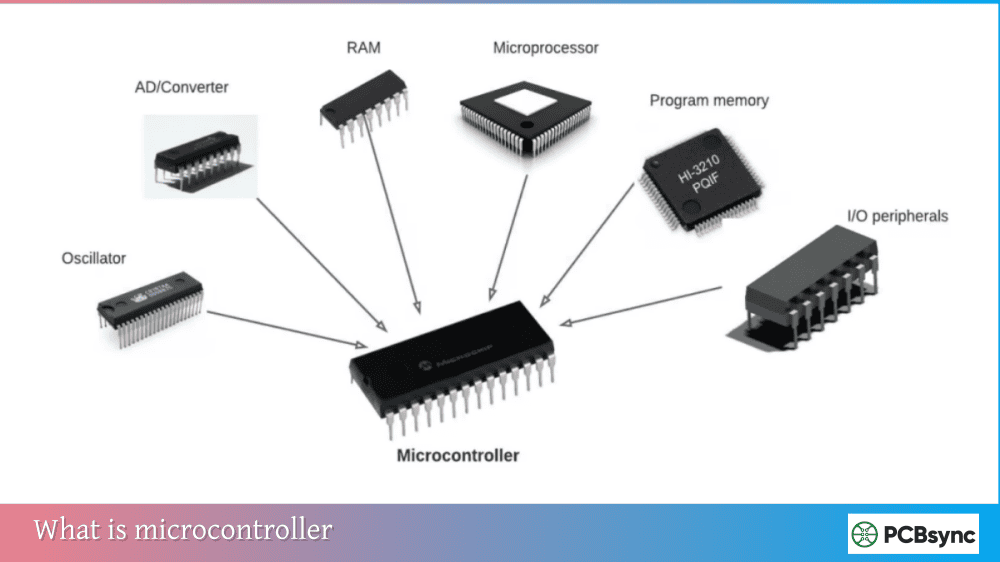
Microcontrollers (MCUs) integrate the processor core with memory (Flash, SRAM) and peripherals (timers, ADCs, communication interfaces) on a single chip. This integration makes MCUs ideal for embedded applications where cost, power, and board space matter more than raw performance.
When selecting a microcontroller, I evaluate peripheral integration first. A $1 MCU with the exact peripherals your application needs beats a $3 MCU requiring external components every time—both for BOM cost and PCB complexity.
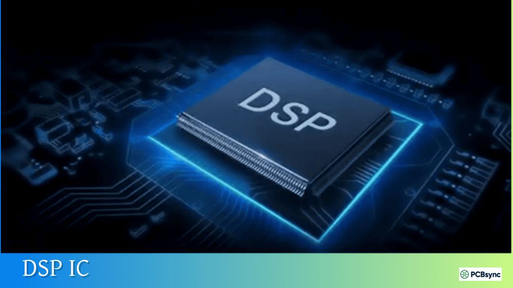
Digital Signal Processors (DSPs)
DSPs are specialized processors optimized for mathematical operations common in signal processing: multiply-accumulate (MAC), filtering, and transforms. Hardware multipliers, specialized addressing modes, and circular buffer support distinguish DSPs from general-purpose processors.
Key DSP features include single-cycle MAC operations, Harvard architecture with separate program and data memories, specialized addressing for FFT butterflies and FIR filters, and saturating arithmetic that clips rather than wraps on overflow.
Applications include audio processing, telecommunications, image processing, radar, software-defined radio, and control systems requiring real-time mathematical operations. Texas Instruments’ C2000 and C6000 families, Analog Devices’ SHARC and Blackfin, and various ARM Cortex-M with DSP extensions represent common choices.
Programmable Logic Devices
Programmable logic represents one of the most significant developments in digital design. Rather than selecting fixed-function ICs, you configure general-purpose silicon to implement your specific logic function.
PAL/GAL (Programmable Array Logic): Early programmable devices with AND-OR structures. PALs were one-time programmable; GALs added electrical erasure. Largely obsolete but occasionally encountered in legacy systems.
CPLD (Complex Programmable Logic Device): Non-volatile programmable logic with predictable timing. CPLDs offer instant-on operation and deterministic propagation delays—valuable for timing-critical glue logic. Internal architecture uses product-term macrocells. Popular families include Xilinx CoolRunner and Intel MAX series.
FPGA (Field-Programmable Gate Array): The most flexible programmable logic, containing thousands to millions of configurable logic blocks, memory, and often specialized functions like DSP blocks and high-speed transceivers. FPGAs implement arbitrary digital logic through look-up tables (LUTs) and programmable interconnect.
Device Type
Configuration
Density
Timing
Power-On
Typical Cost
CPLD
Non-volatile (Flash)
32-512 macrocells
Predictable
Instant
$1-10
SRAM FPGA
Volatile (external config)
1K-2M+ LUTs
Route-dependent
10-500ms
$5-5000
Flash FPGA
Non-volatile (Flash)
1K-100K LUTs
Moderate
Instant
$5-200
FPGAs have transformed hardware development by enabling software-like iteration on hardware designs. Where an ASIC requires months of development and millions in tooling, an FPGA lets you test and revise hardware implementations in hours.
Modern FPGAs include hard IP blocks: embedded ARM processors, DDR memory controllers, PCIe interfaces, and multi-gigabit transceivers. These hybrid devices blur the line between FPGA and SoC.
Application-Specific Integrated Circuits (ASICs)
ASICs are custom-designed chips optimized for a specific application. While FPGAs offer flexibility, ASICs provide superior performance, power efficiency, and per-unit cost at high volumes.
ASIC Types:
Full Custom: Every transistor placement optimized by the design team. Maximum performance and minimum area but highest development cost and time. Used for high-volume, performance-critical chips like smartphone processors.
Standard Cell: Uses pre-designed logic cells from a library, placed and routed by automated tools. Balances customization with development efficiency. Most common ASIC approach.
Gate Array: Partially fabricated wafers with uncommitted transistors. Final metal layers complete the customization. Faster turnaround than standard cell at some cost in density.
Structured ASIC: Combines aspects of gate arrays and FPGAs. Pre-characterized blocks reduce design complexity while maintaining ASIC benefits.
For most projects, the FPGA vs. ASIC decision comes down to volume. Below roughly 10,000 units, FPGA non-recurring engineering (NRE) advantages typically win. Above 100,000 units, ASIC per-unit cost advantages dominate. The crossover point depends heavily on device complexity and performance requirements.
Selecting Digital ICs for Your Design
After covering the types of digital IC available, let me share the practical selection process I use for PCB designs.
Power Budget Considerations
Start with your power budget. Battery-powered devices demand low-power CMOS; industrial equipment with adequate power supplies offers more flexibility.
Calculate both static and dynamic power consumption:
Static power: Leakage currents, always present regardless of activity
Dynamic power: P = CV²f (capacitance × voltage squared × frequency)
Modern CMOS static power is negligible for most applications—typically nanowatts per gate. Dynamic power dominates, making frequency and supply voltage the primary optimization targets. Reducing voltage from 5V to 3.3V cuts dynamic power by 56% (proportional to V²).
Speed Requirements
Match logic family speed to your actual requirements—not to hypothetical future needs. Faster logic families cost more, consume more power, generate more EMI, and require more careful PCB layout.
If your signals change at 1 MHz, 74HC logic with 8ns propagation delays provides enormous timing margin. You don’t need—and shouldn’t use—ECL or advanced BiCMOS unless your application genuinely requires nanosecond timing.
Interface Compatibility
Mixing logic families requires attention to voltage thresholds. A 3.3V CMOS output might not reliably drive a 5V TTL input because TTL requires 2.0V minimum for logic HIGH, while 3.3V CMOS outputs may only guarantee 2.4V.
Use level shifters or select compatible families:
74HCT: 5V CMOS with TTL-compatible inputs
74LVC with 5V tolerant inputs: 3.3V logic accepting 5V signals
Dedicated level translator ICs for mixed-voltage systems
PCB Design Considerations for Digital ICs
Digital IC selection directly impacts your PCB layout strategy.
Power Distribution
Every digital IC needs clean power. For CMOS devices, place a 0.1µF ceramic capacitor within 5mm of each VCC pin. High-speed or high-current devices may need additional bulk capacitance (10µF or more) nearby.
Use solid ground planes—never route signals through ground plane gaps. Return current must flow, and gaps force it to take longer paths, creating EMI and signal integrity problems.
Signal Integrity
Fast edge rates in modern logic create transmission line effects even on short traces. When trace length exceeds roughly one-sixth of the signal’s rise time (in distance), treat it as a transmission line.
Frequently Asked Questions About Digital Integrated Circuits
What is the difference between digital and analog integrated circuits?
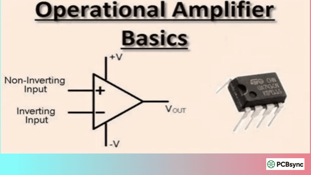
Digital ICs process discrete binary signals (HIGH and LOW voltage levels representing 1s and 0s), while analog ICs handle continuous signals that vary smoothly over a range of values. Digital ICs include logic gates, microprocessors, and memory chips. Analog ICs include operational amplifiers, voltage regulators, and ADCs/DACs. The distinction matters for design: digital circuits focus on timing and logic correctness, while analog circuits prioritize gain, bandwidth, and noise performance. Some modern chips combine both—these mixed-signal ICs handle analog inputs (like sensor data) and produce digital outputs (like I²C or SPI data streams). Understanding this distinction helps you partition system functionality appropriately between digital processing and analog signal conditioning.
Why has CMOS replaced TTL in most modern designs?
CMOS consumes dramatically less power than TTL, particularly at lower operating frequencies. While both technologies now offer comparable speed performance, CMOS draws current primarily during switching transitions rather than continuously. For battery-powered devices, this difference is decisive—a CMOS logic chip might consume microwatts where an equivalent TTL chip draws milliwatts. CMOS also scales better to lower supply voltages (1.8V or even 1.2V versus TTL’s fixed 5V requirement), enabling higher integration densities and reduced power consumption in VLSI designs. The only areas where TTL variants still appear are legacy system support, some educational applications, and specific high-current drive situations where TTL’s stronger output stage offers advantages without requiring external buffering.
When should I use an FPGA versus a microcontroller?
Choose a microcontroller when your application involves sequential processing, the timing requirements are modest (microseconds rather than nanoseconds), and software flexibility matters. Microcontrollers excel at control logic, user interfaces, and communication protocols where the software approach simplifies development and maintenance. Choose an FPGA when you need massive parallelism (processing many signals simultaneously), deterministic nanosecond-level timing, or hardware interfaces not available in any microcontroller. FPGAs also make sense for prototyping custom digital hardware before ASIC development or when production volumes don’t justify ASIC tooling costs. Many modern designs combine both approaches: an FPGA handling high-speed signal processing with a microcontroller managing system configuration, user interface, and network communication. Some devices (like Xilinx Zynq) integrate both on a single chip.
What determines the integration level (SSI, MSI, LSI, VLSI) of a digital IC?
Integration level describes transistor count and complexity, reflecting manufacturing capability at different points in semiconductor history. SSI (Small Scale Integration) devices contain up to 100 transistors implementing a few logic gates—the original integrated circuits of the 1960s. MSI (Medium Scale Integration) reaches 1,000 transistors, enabling multiplexers, counters, and similar functions. LSI (Large Scale Integration) extends to 10,000 transistors—enough for simple microprocessors and small memories. VLSI (Very Large Scale Integration) encompasses 10,000 to 1 million transistors, covering advanced processors and larger memories. ULSI (Ultra Large Scale Integration) describes modern chips exceeding 1 million transistors. Current smartphone processors contain over 10 billion transistors—the terminology struggles to keep pace with Moore’s Law progress. Practically, these terms now mostly appear in educational contexts and historical discussions; working designers focus on device function and specifications rather than transistor count.
How do I interface different logic families operating at different voltages?
Several approaches work depending on the specific voltage combination and performance requirements. For 5V to 3.3V conversion, many 3.3V CMOS devices accept 5V inputs directly—check datasheets for “5V tolerant” specifications on input pins. Simple resistor dividers also work for slow signals. Going from 3.3V to 5V typically requires active level shifting since 3.3V outputs may not reach TTL HIGH thresholds reliably. Dedicated level translator ICs (like TXB0108 for bidirectional translation or 74LVC4245 for bus interfaces) handle this cleanly with minimal propagation delay. For simple unidirectional signals, a MOSFET level shifter provides a low-cost solution. When mixing 1.8V and 3.3V logic, similar considerations apply with appropriate device selection. Always verify that your chosen solution handles the actual signal speed requirements—some level shifters introduce significant propagation delays that may affect high-speed interfaces like SPI or I²C at higher clock rates.
Conclusion: Selecting the Right Digital IC for Your Application
Understanding types of digital IC and their characteristics enables informed component selection for any electronics project. From simple 74HC logic gates providing glue logic on a control board to billion-transistor processors powering smartphones, digital integrated circuits form the foundation of modern electronics.
The key takeaways from this digital IC guide:
Logic family selection (TTL, CMOS, ECL, BiCMOS) determines power consumption, speed, and interface requirements. For new designs, CMOS variants (74HC, 74LVC) typically offer the best balance of performance, power efficiency, and cost.
Integration level has progressed from SSI devices with a handful of gates to ULSI chips containing billions of transistors. This progression continues enabling more functionality in smaller, cheaper, lower-power packages every year.
Programmable logic (CPLDs and FPGAs) has transformed digital design by enabling hardware iteration at software-development speeds, while ASICs remain essential for high-volume, performance-critical applications where maximum efficiency justifies development investment.
Every selection involves tradeoffs—there’s no universally “best” digital IC, only the right choice for your specific requirements. Define your power budget, speed requirements, interface needs, and volume expectations before selecting components, and you’ll build more reliable, cost-effective designs.
The digital IC landscape continues evolving rapidly. New process nodes, advanced packaging technologies like chiplets, and emerging memory technologies promise continued performance improvements. Staying current with these developments ensures you leverage the best available technology for each new design challenge.
Inquire: Call 0086-755-23203480, or reach out via the form below/your sales contact to discuss our design, manufacturing, and assembly capabilities.
Quote: Email your PCB files to Sales@pcbsync.com (Preferred for large files) or submit online. We will contact you promptly. Please ensure your email is correct.
Notes: For PCB fabrication, we require PCB design file in Gerber RS-274X format (most preferred), *.PCB/DDB (Protel, inform your program version) format or *.BRD (Eagle) format. For PCB assembly, we require PCB design file in above mentioned format, drilling file and BOM. Click to download BOM template To avoid file missing, please include all files into one folder and compress it into .zip or .rar format.


